Grid Search Hyperparameter optimization
This case study is all about using grid searches to identify the optimal parameters for a machine learning algorithm. To complere this case study, you'll use the Pima Indian diabetes dataset from Kaggle and KNN. Follow along with the preprocessing steps of this case study.
Load the necessary packages
import numpy as np
import pandas as pd
import matplotlib.pyplot as plt
import seaborn as sns
sns.set()

# set random seed to try make this exercise and solutions reproducible (NB: this is just for teaching purpose and not something you would do in real life)
random_seed_number = 42
np.random.seed(random_seed_number)
Load the diabetes data
diabetes_data = pd.read_csv('data/diabetes.csv')
diabetes_data.head()
Start by reviewing the data info.
diabetes_data.info()
Apply the describe function to the data.
diabetes_data.describe()
Currently, the missing values in the dataset are represented as zeros. Replace the zero values in the following columns ['Glucose','BloodPressure','SkinThickness','Insulin','BMI'] with nan .
diabetes_data[['Glucose','BloodPressure','SkinThickness','Insulin','BMI']] = diabetes_data[['Glucose','BloodPressure','SkinThickness','Insulin','BMI']].replace({0:np.nan,'0':np.nan})

diabetes_data.head()
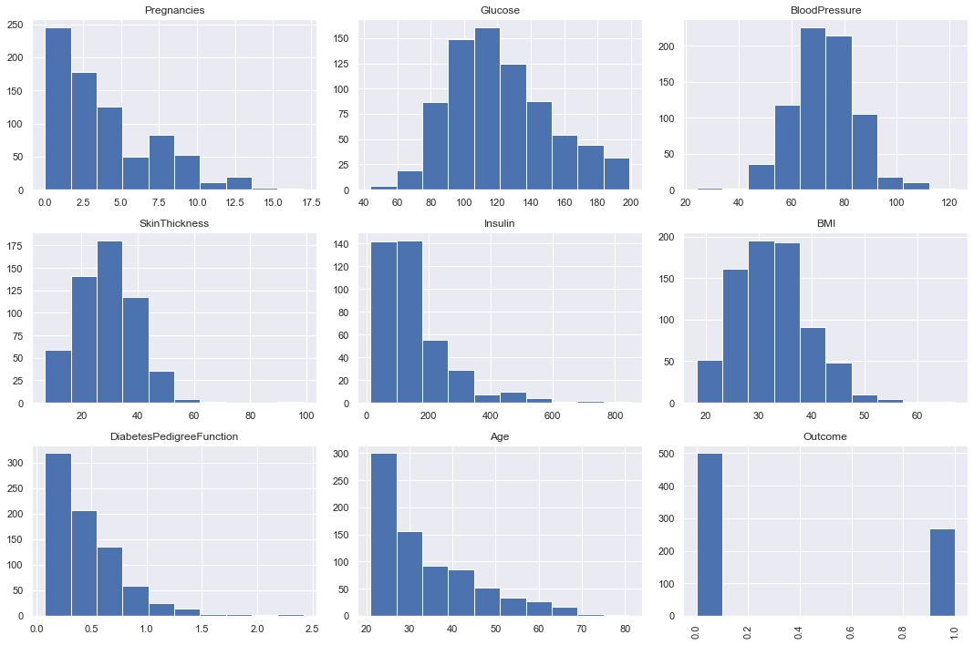
Plot histograms of each column.
diabetes_data.hist(figsize=(15,10))
plt.subplots_adjust(hspace=0.2)
plt.xticks(rotation='vertical')
plt.tight_layout()
plt.show();
Replace the zeros with mean and median values.
diabetes_data['Glucose'].fillna(diabetes_data['Glucose'].mean(), inplace = True)
diabetes_data['BloodPressure'].fillna(diabetes_data['BloodPressure'].mean(), inplace = True)
diabetes_data['SkinThickness'].fillna(diabetes_data['SkinThickness'].median(), inplace = True)
diabetes_data['Insulin'].fillna(diabetes_data['Insulin'].median(), inplace = True)
diabetes_data['BMI'].fillna(diabetes_data['BMI'].median(), inplace = True)
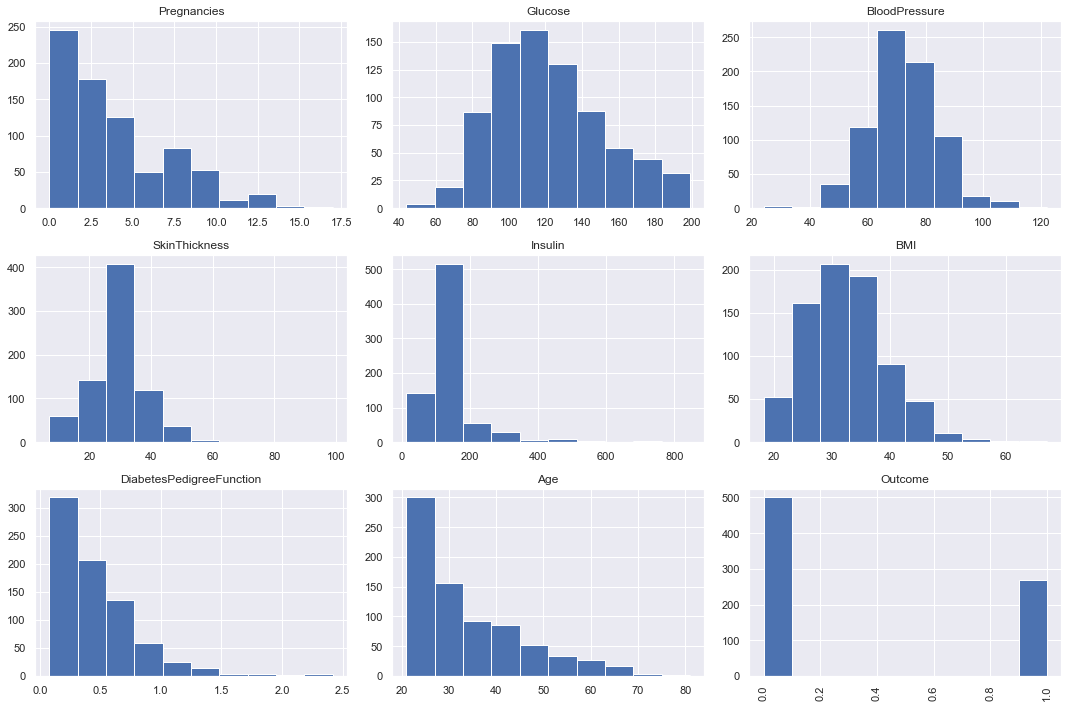
Plot histograms of each column after replacing nan.
diabetes_data.hist(figsize=(15,10))
plt.subplots_adjust(hspace=0.2)
plt.xticks(rotation='vertical')
plt.tight_layout()
plt.show();
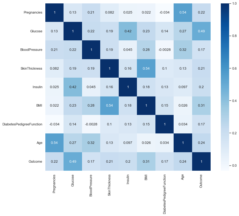
Plot the correlation matrix heatmap
plt.figure(figsize=(12,10))
print('Correlation between various features')
p=sns.heatmap(diabetes_data.corr(), annot=True,cmap ='Blues')
Define the `y` variable as the `Outcome` column.
y = diabetes_data.Outcome
Create a 70/30 train and test split.
X = diabetes_data.drop('Outcome',axis=1)

# Train Test split
from sklearn.model_selection import train_test_split

X_train, X_test, y_train, y_test = train_test_split(X, y, test_size=0.3, random_state=42)
Using Sklearn, standarize the magnitude of the features by scaling the values.
Note: Don't forget to fit() your scaler on X_train and then use that fitted scaler to transform() X_test. This is to avoid data leakage while you standardize your data.
# Scale
from sklearn.preprocessing import StandardScaler, MinMaxScaler
scaler = StandardScaler()
X_train = scaler.fit_transform(X_train)
X_test = scaler.transform(X_test)
X_train.shape
Using a range of neighbor values of 1-10, apply the KNearestNeighbor classifier to classify the the data.
from sklearn.neighbors import KNeighborsClassifier


test_scores = []
train_scores = []

for i in range(1,10):

    knn = KNeighborsClassifier(i)
    knn.fit(X_train,y_train)

    train_scores.append(knn.score(X_train,y_train))
    test_scores.append(knn.score(X_test,y_test))
Print the train and test scores for each iteration.
for i in range(len(test_scores)):
    if i == 0:
        print('k\tTrain_scores\tTest_scores')
    print(f'{i+1}\t{train_scores[i]: .5f}\t{test_scores[i]: .5f}')
Identify the number of neighbors that resulted in the max score in the training dataset.
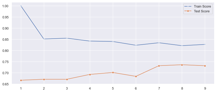
The train_scores is the best when k equals 1.
Identify the number of neighbors that resulted in the max score in the testing dataset.
The test_scores is the best when k equals 8.
Plot the train and test model performance by number of neighbors.
plt.figure(figsize=(12,5))
p = sns.lineplot(range(1,10),train_scores,marker='*',label='Train Score')
p = sns.lineplot(range(1,10),test_scores,marker='o',label='Test Score')
Fit and score the best number of neighbors based on the plot.
knn = KNeighborsClassifier(8)
knn.fit(X_train,y_train)
from sklearn.metrics import confusion_matrix
y_pred = knn.predict(X_test)
pl = confusion_matrix(y_test,y_pred)
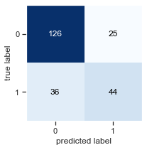
Plot the confusion matrix for the model fit above.
from mlxtend.plotting import plot_confusion_matrix
fig, ax = plot_confusion_matrix(conf_mat=confusion_matrix(y_test,y_pred), figsize=(3, 3))
plt.show()
Print the classification report
from sklearn.metrics import confusion_matrix,classification_report
# print(confusion_matrix(y_test,y_pred))
print(classification_report(y_test,y_pred))
In the case of the K nearest neighbors algorithm, the K parameter is one of the most important parameters affecting the model performance. The model performance isn't horrible, but what if we didn't consider a wide enough range of values in our neighbors for the KNN? An alternative to fitting a loop of models is to use a grid search to identify the proper number. It is common practice to use a grid search method for all adjustable parameters in any type of machine learning algorithm. First, you define the grid — aka the range of values — to test in the parameter being optimized, and then compare the model outcome performance based on the different values in the grid.
Run the code in the next cell to see how to implement the grid search method for identifying the best parameter value for the n_neighbors parameter. Notice the param_grid is the range value to test and we apply cross validation with five folds to score each possible value of n_neighbors.
from sklearn.model_selection import GridSearchCV
param_grid = {'n_neighbors':np.arange(1,50)}
knn = KNeighborsClassifier()
knn_cv= GridSearchCV(knn,param_grid,cv=5)
knn_cv.fit(X,y)
Print the best score and best parameter for n_neighbors.
print("Best Score:" + str(knn_cv.best_score_))
print("Best Parameters: " + str(knn_cv.best_params_))
Here you can see that the ideal number of n_neighbors for this model is 14 based on the grid search performed.
Now, following the KNN example, apply this grid search method to find the optimal number of estimators in a Randon Forest model.
from sklearn.ensemble import RandomForestClassifier
param_grid = {'n_neighbors':np.arange(1,50)}
rfc = RandomForestClassifier(n_estimators=600)
rfc_cv= GridSearchCV(knn,param_grid,cv=5)
rfc_cv.fit(X,y)
print("Best Score:" + str(rfc_cv.best_score_))
print("Best Parameters: " + str(rfc_cv.best_params_))
