Cosine Similarity Calculations
Cosine similarity is a measure of similarity between two non-zero vectors of an inner product space that measures the cosine of the angle between them. Similarity measures have a multiude of uses in machine learning projects; they come in handy when matching strings, measuring distance, and extracting features. This similarity measurement is particularly concerned with orientation, rather than magnitude. In this case study, you'll use the cosine similarity to compare both a numeric data within a plane and a text dataset for string matching.
Load the Python modules, including cosine_similarity, from sklearn.metrics.pairwise
import numpy as np
import pandas as pd
import matplotlib.pyplot as plt
import matplotlib.cm as cm
%matplotlib inline
plt.style.use('ggplot')
from scipy import spatial
from sklearn.metrics.pairwise import cosine_similarity
Load the distance dataset into a dataframe.
df = pd.read_csv('distance_dataset (1).csv')
df.head()
Cosine Similarity with clusters and numeric matrices
All points in our dataset can be thought of as feature vectors. We illustrate it here as we display the Cosine Similarity between each feature vector in the YZ plane and the [5, 5] vector we chose as reference. The sklearn.metrics.pairwise module provides an efficient way to compute the cosine_similarity for large arrays from which we can compute the similarity.
First, create a 2D and a 3D matrix from the dataframe. The 2D matrix should contain the 'Y' and 'Z' columns and the 3D matrix should contain the 'X','Y', and 'Z' columns.
import cufflinks as cf

cf.set_config_file(sharing='public',theme='pearl',offline=False)
cf.go_offline()
df.iplot(kind='scatter',x='Y',y='Z',
         xTitle='X',
         yTitle='Y',
         mode='markers',
         size=10
        )
df.iplot(kind='scatter3d',
        x='X',
        y='Y',
        z='Z',
        xTitle='X',
        yTitle='Y',
        zTitle='Z',
        size=15,
#         categories='categories',
#         text='text',
        title='Cufflinks - Scatter 3D Chart',
        colors=['blue'],
        width=0.5,
        margin=(0,0,0,0),
        opacity=1)
Calculate the cosine similarity for those matrices with reference planes of 5,5 and 5,5,5. Then subtract those measures from 1 in new features.
mat = np.array(df[['X','Y','Z']]).copy()
matYZ = df[['Y','Z']].copy()
simCosine3D = 1. - cosine_similarity(mat, [[5,5,5]], 'cosine')
simCosine = 1. - cosine_similarity(matYZ, [[5,5]], 'cosine')
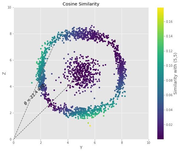
Using the 2D matrix and the reference plane of (5,5) we can use a scatter plot to view the way the similarity is calculated using the Cosine angle.
figCosine = plt.figure(figsize=[10,8])

plt.scatter(df.Y, df.Z, c=simCosine[:,0], s=20)
plt.plot([0,5],[0,5], '--', color='dimgray')
plt.plot([0,3],[0,7.2], '--', color='dimgray')
plt.text(0.7,2.6,r'$\theta$ = 22.4 deg.', rotation=47, size=14)
plt.ylim([0,10])
plt.xlim([0,10])
plt.xlabel('Y', size=14)
plt.ylabel('Z', size=14)
plt.title('Cosine Similarity')
cb = plt.colorbar()
cb.set_label('Similarity with (5,5)', size=14)

#figCosine.savefig('similarity-cosine.png')
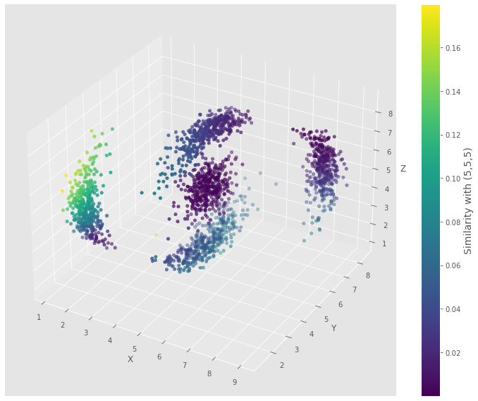
Now, plot the 3D matrix with the similarity and the reference plane, (5,5,5).
from mpl_toolkits.mplot3d import Axes3D

figCosine3D = plt.figure(figsize=(10, 8))
ax = figCosine3D.add_subplot(111, projection='3d')

p = ax.scatter(mat[:,0], mat[:,1], mat[:,2], c=simCosine3D[:,0])
ax.set_xlabel('X')
ax.set_ylabel('Y')
ax.set_zlabel('Z')
cb = figCosine3D.colorbar(p)
cb.set_label('Similarity with (5,5,5)', size=14)

figCosine3D.tight_layout()
#figCosine3D.savefig('cosine-3D.png', dpi=300, transparent=True)
Cosine Similarity with text data
This is a quick example of how you can use Cosine Similarity to compare different text values or names for record matching or other natural language proecessing needs. First, we use count vectorizer to create a vector for each unique word in our Document 0 and Document 1.
from sklearn.feature_extraction.text import CountVectorizer
count_vect = CountVectorizer()
Document1 = "Starbucks Coffee"
Document2 = "Essence of Coffee"

corpus = [Document1,Document2]

X_train_counts = count_vect.fit_transform(corpus)
print(X_train_counts)

pd.DataFrame(X_train_counts.toarray(),columns=count_vect.get_feature_names(),index=['Document 0','Document 1'])
Now, we use a common frequency tool called TF-IDF to convert the vectors to unique measures.
from sklearn.feature_extraction.text import TfidfVectorizer
vectorizer = TfidfVectorizer()
trsfm=vectorizer.fit_transform(corpus)
pd.DataFrame(trsfm.toarray(),columns=vectorizer.get_feature_names(),index=['Document 0','Document 1'])
trsfm
Here, we finally apply the Cosine Similarity measure to calculate how similar Document 0 is compared to any other document in the corpus. Therefore, the first value of 1 is showing that the Document 0 is 100% similar to Document 0 and 0.26055576 is the similarity measure between Document 0 and Document 1.
cosine_similarity(trsfm[0:1], trsfm)
Replace the current values for Document 0 and Document 1 with your own sentence or paragraph and apply the same steps as we did in the above example.
Combine the documents into a corpus.
doc3 = ' anniversary, and to celebrate and recognize 50 grateful years bringing communities together over coffee Starbucks is inviting customers to bring in a clean, empty, reusable cup (up to 20 fl. oz.) into participating café locations in Canada on September 29 and get a free cup of Pike Place® Roast brewed coffee*.'
doc4 = 'Named after the location of the original store in Seattle’s Pike Place Market that opened in 1971, Pike Place Roast is Starbucks signature medium roast coffee served in stores everyday around the world. '

# These doc3 and doc4 are from https://stories.starbucks.ca/en/stories/2021/starbucks-celebrates-its-50th-anniversary-on-national-coffee-day-with-free-coffee/

corpus = [doc3,doc4]
Apply the count vectorizer to the corpus to transform it into vectors.
X_train_counts = count_vect.fit_transform(corpus)
# print(X_train_counts)
Convert the vector counts to a dataframe with Pandas.
pd.DataFrame(X_train_counts.toarray(),
             columns=count_vect.get_feature_names(),index=['Document 3','Document 4'])
Apply TF-IDF to convert the vectors to unique frequency measures.
vectorizer = TfidfVectorizer()
trsfm=vectorizer.fit_transform(corpus)
pd.DataFrame(trsfm.toarray(),columns=vectorizer.get_feature_names(),index=['Document 3','Document 4'])
Use the cosine similarity function to get measures of similarity for the sentences or paragraphs in your original document.
cosine_similarity(trsfm[0:1], trsfm)